Regular and Computed Booleans in MySQL
A comparison between regular boolean fields and MySQL's Computed Columns along the rationale behind changes in our codebase
TL;DR: In our tests, transitioning from a table that only has an is_deleted
field to a table that includes both a deleted_at field provided at write-time
and a computed is_deleted field stored by the database server results in
approximately an 8% increase in table size and a 2% decrease in SELECT
performance. We decided to make the switch due
to its positive effect on developer ergonomics and the intricate balance
between technical and human aspects of Software Engineering.
At Doist, our backend use soft deletes in some of our models to retain some historical data.
Similar to what is commonly done in situations like this, we have traditionally
used boolean flags, such as is_deleted, to denote whether a record is
considered deleted or not. That boolean-flag-based structure is useful
for any kind of scenario where a record’s state needs to be stored in
the record itself, though it is not the only viable option for this.
Recently, we have evaluated using timestamp-based flags, such as deleted_at in
order to have a temporal marking of when a given record entered a state.
As interesting as this may be, swapping a pure boolean field for one
that handles dates and times is not without its cost. An alternative
to having only a timestamp such as deleted_at is to have both a
timestamp and a boolean field that is computed by the server
and used to speed up queries.
How it is now – we only know if a record is or isn’t deleted:
>>> row = Row(data)
>>> row.is_deleted # False

Row.find(...) # by default, filters-out rows with is_deleted = True

def delete(row):
    row.is_deleted = True
    # Save and commit to the database
What we wanted – knowing if a record is or isn’t deleted and when it was deleted:
row = Row(data)
row.deleted_at # None, by default

Row.find(...) # Ignores rows with deleted_at != None

def delete(row):
    row.deleted_at = datetime.utcnow()
    # Save and commit
In this post, we’ll discuss the benefits and drawbacks of each approach, how we tested and evaluated them, and why we choose to move to timestamp fields with stored booleans, even though they have a small performance hit.
Boolean Flags & Date Time Records
Booleans are small pieces of data that only have two possible values: True and
False (or, jokingly, FileNotFound, according to
this gem of Internet History).
Dates and times, however, have a wide range of possible values. If we consider
a resolution based on seconds alone, we have well over 30 million possible values.
This measurement of the possible size of a given set is known as the set’s
cardinality, and it is an important concept when analyzing and predicting
database performance. Before doing any such migration, we were interested
in evaluating its impact on query performance. It is critical to note
that if a model supports soft-deletes, almost every query
will involve a filter like WHERE NOT is_deleted.
Touching a database column that is so commonly used around a system cannot be taken lightly. If we have a performance hit in one of those areas, it can quickly spread everywhere.
Apart from the sheer time that a given query occurs, another important metric to keep in mind is the on-disk storage size of a given table and its indexes. Datetimes are bigger than booleans by their own nature, so we expected an overall increase in those metrics.
Generate Columns
Broadly speaking, MySQL’s generated columns are calculated by the database server at some point in time – it can be at insert or at select-time, for example. Those columns differ by yet another case – if they are stored or not.
In MySQL parlance, we have the following nomenclature:
| Column Type | Computed At | Stored? |
|---|---|---|
VIRTUAL | SELECT, when rows are read | No |
STORED | INSERT/UPDATE, on writes | Yes |
Stored computed columns are the ones we were most interested in. They would
allow us to, for example, calculate a boolean is_deleted based on whether
the deleted_at column is or isn’t null. Having the server calculate
this means that we can let our developers not care about providing
values to this boolean column, but have it in place
and leverage it in queries.
Experimental Setup
We tested four different table structures:
- Pure Boolean (Table A): A table with a simple
is_deletedcolumn that is indexed, similar to our current implementation. - Pure Timestamps, not-indexed (Table B): A table with a
deleted_atdatetime column without an index - Pure Timestamps, indexed (Table C): A table with a
deleted_atdatetime column with an index. - Timestamps with computed booleans (Table D): A table with a
deleted_atdatetime column without an index and a virtual, stored, boolean column is_deleted that holds the value ifdeleted_atis or isn’t null. This column is indexed.
We created these tables and populated them with varying numbers of rows (1, 100, 1,000, 10,000, and 100,000) with randomized timestamps. We then measured the time taken for insert operations and various select queries using both Python-based tools and MySQL.
Summary of Results
We can conclude:
- Overall, the performance impact between pure booleans and computed booleans
was small enough that we have a case to use computed columns to replace the current
is_deletedfield. - Pure booleans are more performant than datetimes or computed booleans, as expected.
- For most analyses, though, there is no clear-cut difference between pure booleans, indexed date times, and computed booleans. Most differences are in the single-digit percentages.
- Index size is the main factor that makes computed booleans more favorable than indexing date times. While indexed datetimes showed good performance, they also resulted in a bigger index size. This is expected, given the higher cardinality of datetimes.
Insert Performance
Results from %timeit calls. Inserts were not batched to reflect better our regular usage, in which queries happen in isolation. This data represents a statistic based on 7 runs:
| Records | Boolean (Table A) | Timestamp, Not Indexed (Table B) | Timestamp, Indexed (Table C) | Timestamp Not Indexed + Computed Boolean (Table D) |
|---|---|---|---|---|
| 100 | 96.8ms ± 1.16ms | 96.1ms ± 1.05ms | 109ms ± 2.86ms | 102ms ± 1.57ms |
| 1,000 | 1.05s ± 27.5ms | 961ms ± 9.29ms | 1.03s ± 51.3 ms | 1s ± 6.66ms |
| 10,000 | 10.5s ± 310.5ms | 10.02s ± 82.3ms | 9.94s± 490.2 ms | 11.5s ± 65.6ms |
We can see that inserting values to an indexed timestamp field is not significantly more costly than inserting data to a pure boolean field. The same can be said about computed booleans vs pure booleans.
While the data show small differences, the results are close enough that we cannot safely say that any one method is absolutely more performant than the other, while considering the timing aspects alone.
Length Statistics
The tables were filled with a total of 500k random records each. The data below was reported by MySQL:
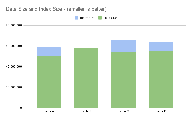
Data statistics from MySQL
data_length | index_length | |
|---|---|---|
| Pure Booleans (Table A) | 50,937,856 | 7,880,704 |
| Non-indexed Timestamps (Table B) | 58,294,272 | 0 |
| Indexed Timestamps (Table C) | 54,099,968 | 12,075,008 |
| Timestamps with Virtual Boolean (Table D) | 55,148,544 | 8,929,280 |
After inserting the records, some differences become clearer. As expected, indexed timestamps are the biggest indexes by far. As a matter of fact, the cardinality of the index for the timestamp field was 241,818.
The table with a computed column (table D) had the second-biggest index, about 13% bigger than standard booleans (table A). Besides that, the table with the computed columns was also bigger than the one without them (table C), which is expected as we are now keeping an additional value.
All in all, using the computed column increased the table size by ~8% when compared to pure booleans and by ~2% when compared with timestamps with indexes but without the computed column. Overall, adding up data and index lengths, the combination of timestamp and computed boolean resulted in a table that is ~8% bigger than the one with just the boolean column (Table D vs Table A).
An interesting, parallel fact to note comes from comparing the table with indexed timestamps (table C) with the table with the computed boolean (table D). This shows that using indexed timestamps creates a table that is about 3.2% bigger. A finding showcasing the impact that a higher-cardinality index has on the overall size. The table with the computed column stores more data than the one with just the timestamp field and index, but it ends up being smaller.
Select Performance
Count — Python
All selects executed were SELECT COUNT(*) filtering for deleted rows. All tables had 500k rows. Timings are done with %timeit, results represent 7 runs:
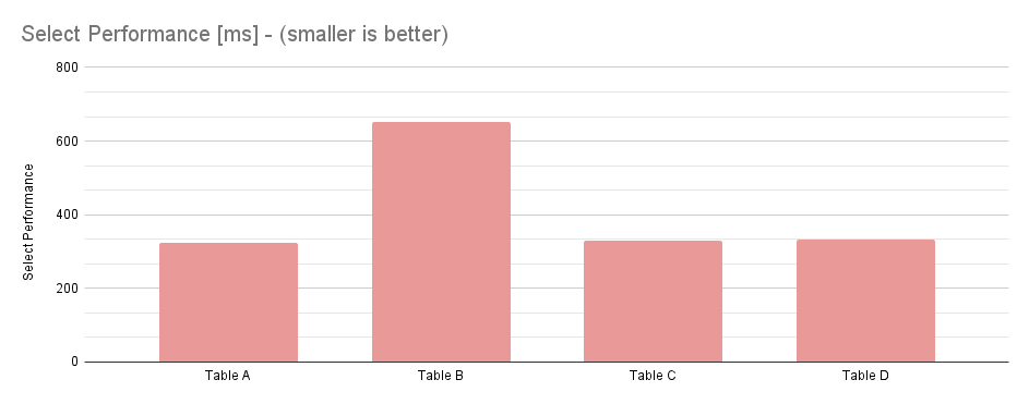
Select performance data
| Boolean (Table A) | Timestamp, Not Indexed (Table B) | Timestamp, Indexed (Table C) | Timestamp Not Indexed + Computed Boolean (Table D) |
|---|---|---|---|
| 304 ms ± 683 µs | 604 ms ± 1.54 ms | 312 ms ± 844 µs | 310 ms ± 791 µs |
Count — MySQL
| Boolean (Table A) | Timestamp, Not Indexed (Table B) | Timestamp, Indexed (Table C) | Timestamp Not Indexed + Computed Boolean (Table D) |
|---|---|---|---|
| 325 ms | 652 ms | 329 ms | 333 ms |
Based on both datasets, pure boolean queries rank as the most performant, and queries on the indexed timestamp and computed boolean tables are close to a tie. Considering the averaged timings, computed booleans (Table D) were ~2% slower than pure booleans (Table A)
Query Cost — MySQL
As reported by last_query_cost :
| Boolean (Table A) | Timestamp, Not Indexed (Table B) | Timestamp, Indexed (Table C) | Timestamp Not Indexed + Computed Boolean (Table D) |
|---|---|---|---|
| 45,198.119732 | 103,365.599000 | 47,476.020162 | 47,309.717293 |
Similar to select performance, pure boolean is a clear winner, and both indexed and computed booleans are very close together. The difference between pure booleans (Table A) and computed booleans (Table D) is ~4%.
It is worth noting that this analysis may be the least significant one, as query cost is more useful to compare different query plans for a similar query, and not between different queries altogether.
DB Performance & Developer Experience
Besides performance, an important feature of any system that is intended to be maintained over a long period of time is developer experience. This matters very much in our case as Todoist is a codebase that is both a decade old and where we’re just starting out.
When software engineering-related aspects come into view, more subjective and less clean-cut aspects like maintainability and ergonomics around the code base become more relevant. It is way harder to get a measurable metric for more human-related aspects of software development than it is to analyze technical benchmarks
From a purely technical perspective, making the change to computed booleans does not make much sense. But, from the human side of engineering, it does. Having a timestamp for when a given state was entered allows us to do more interesting and robust debugging and analysis.
The fact that subjective metrics are harder to define and monitor makes them a prime target for under-prioritization. This may not be a problem for prototypes and so on, but it is a problem when dealing with a codebase that we plan to keep sustainable, fun, and productive in the decades to come. At Doist, we proudly stand in the second group.
Balancing Computed Fields vs. Manually Managed Fields
We could have achieved our desired goal of using timestamps when dealing with a state flag and then converting it internally to a second boolean column or even just a boolean-like behavior by patching the code that accesses those data records. This would allow us to not have to deal with any kind of MySQL wizardry related to computing columns based on other columns and so on and so forth! So, why not?
The problem with that approach is that we would have to centralize every access to our tables through some shared code that would do all of this handling. Sometimes we don’t even want or can do that.
Having the database server handling that computation gives us a guarantee that it does not actually matter how a record is written or updated, the relevant boolean flag will always be updated as well, and we won’t find ourselves in a situation where we have a record with a non-null deleted_at field with a false is_deleted flag.
Testing Limitations and Pitfalls
Benchmarking systems is always a tricky endeavor. Several effects parallel to the system under test can skew results and — even when the utmost care is taken to minimize extraneous factors — these effects can still produce biased results.
In our particular case, we were not interested in making a broad, general claim about the absolute performance of one approach or the other. Rather, we were interested in their relative, comparative performance. For our intents and purposes, putting all the approaches under the same experimental setup, helps us get valuable data. We do recognize a few limitations of our approach:
- Tests were executed on the same machine as the DB was running.
- Tests were executed in a single-threaded manner with a single process. While this is useful for comparing strategies, it fundamentally differs from how most system works (single-threaded, multiple processes).
Please be aware of using any benchmark data to support claims that are different than the ones that the benchmark was made to test! This can lead to bogus results.
Bonus: Mixins over SQLAlchemy
With the data presented in the original research, our team set out to define it on an internal spec outlining our findings and how timestamp flags should be dealt with from now on. Our preferred choice of implementation was through mixins on SQLAlchemy. This allows us to easily add the more common soft-deleted columns in any models we like, and also provides us with a boilerplate code on how to implement similar timestamp-as-flag behavior in any other flag we feel like. Here is an example of that, implementing the “SoftDelete” mixin:
from sqlalchemy import Boolean, Column, FetchedValue, func
from sqlalchemy.dialects.mysql import DATETIME
from sqlalchemy.orm import declarative_mixin


@declarative_mixin
class SoftDeletedMixin:
    deleted_at = Column(DATETIME(fsp=6), nullable=True, server_default=None)
    is_deleted = Column(
        Boolean, nullable=False, server_default="0", server_onupdate=FetchedValue()
    )

    @declared_attr
    def __table_args__(cls):
        return (Index(f"idx_is_deleted_{cls.__tablename__}", "is_deleted"),)
We hope that in publishing this article, we contribute back to the wonderful MySQL & SQLAlchemy ecosystems and provide a bit of insight on how we work with technical challenges in our daily tasks.